Oli Thompson

• We programmed a Baxter robot to build a brick well structure. The software used multithreading and image recognition with Python and OpenCV and was tested on a Gazebo physics simulation and the real robot/. My Contribution was writing a computer vision algorithm to align the robot's end effector with the brick, and a path planning algorithm to allow for smooth motion.

Following on from our third year robotics theory module we were able to apply our knowledge to a real robot. We setup a physics simulation using ROS and edited the physical properties of the 3D models to best represent reality. We built a mathematical model of the 7 DOF robot and used this to calculate the joint angles throughout the robot's movement. We implemented redundancy reduction, gripper force detection, path planning and image recognition algorithms to allow the robot to complete its task.

How The Image Recognition Algorithm Works

The computer vision algorithm saves a png frame from the video stream returned from Baxter's wrist camera.

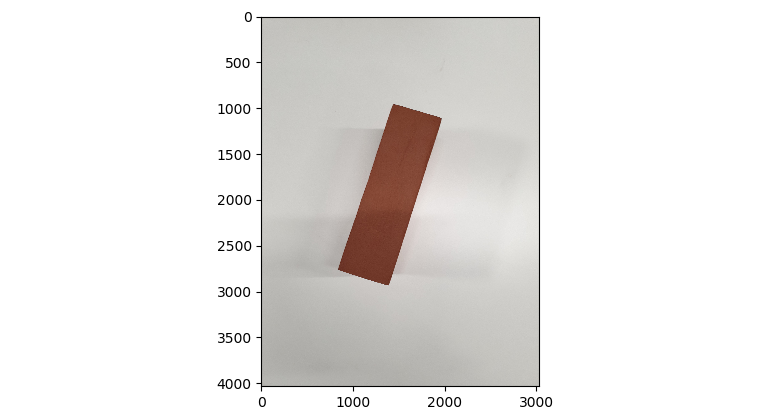
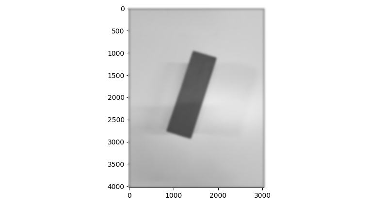
First the image is converted to greyscale to allow the algorithm to run more quickly. A gaussian blur is applied to the image.

gray = cv2.cvtColor(img, cv2.COLOR_BGR2GRAY) #desaturate image
adapt_type = cv2.ADAPTIVE_THRESH_GAUSSIAN_C #threshold value is the weighted sum of neighborhood values where weights are a Gaussian window.

An adaptive threshold edge detection algorithm detects the hard borders between different pixel values. It essentially differentiates the image.

thresh_type = cv2.THRESH_BINARY_INV #define threshold type, hard border between pixels
bin_img = cv2.adaptiveThreshold(blur, 255, adapt_type, thresh_type, 11, 2) #11 is the size of the pixel neighbourhood used to find the threshold value. 2 is the constant subtracted from the mean

From here the 'houghlines' algorithm returns the lines of best fit between all the edge points. The lines are described in Hesse normal form to avoid infinite or zero gradients. The 'cv2.kmeans' algorithm is used to segment the lines into horizontal and vertical, as these are the intersections we are interested in. This is done by multiplying the angle by 2 and comparing it to a unit circle.

 labels, centers = cv2.kmeans(pts, k, None, criteria, attempts, flags)[1:]

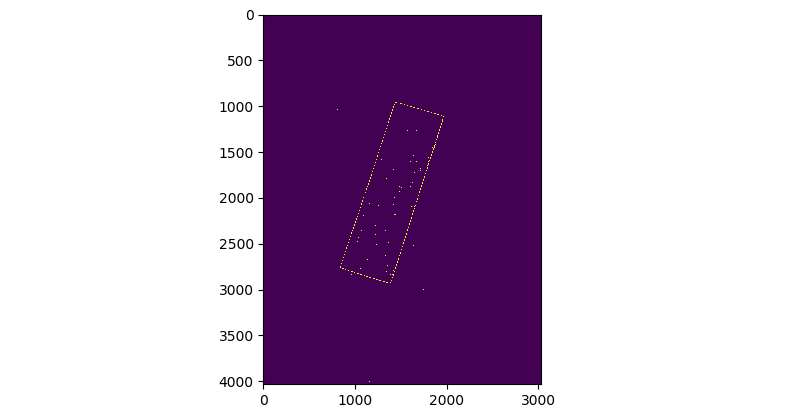
Two further functions, 'intersections' and 'segmented_intersections' use linear algebra to solve the coordinates of each intersection between the segmented lines and arrange them in order. The coordinates of each intersection are plotted using 'matplotlib'.

A = np.array([
[np.cos(theta1), np.sin(theta1)],
[np.cos(theta2), np.sin(theta2)]
])
b = np.array([[rho1], [rho2]])
x0, y0 = np.linalg.solve(A, b)

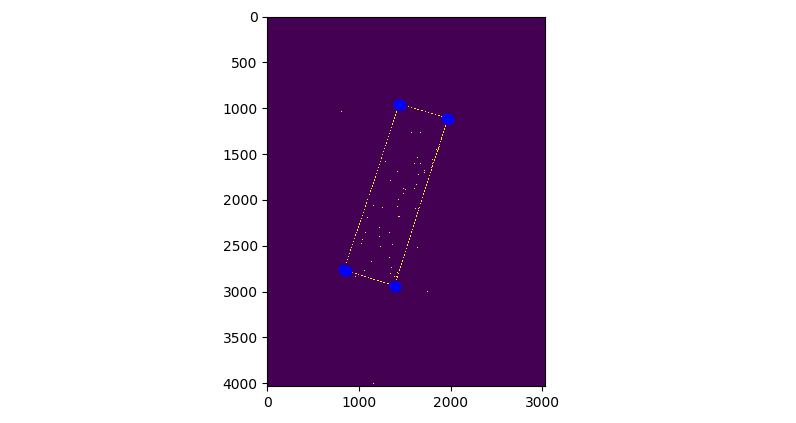
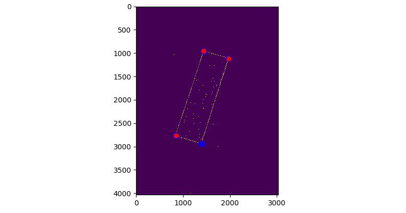
The 'kmeans cluster' function is used to return 4 clusters of the intersections, which accurately correspond to the corners of the brick. One corner is discarded at random as this it is no longer required and the remaining 3 are plotted.

kmeans = KMeans(n_clusters=4, random_state=0).fit(newintersections) #find and return 4 averaged clusters of coordinates

Lines are calculated from the remaining 3 points' coordinates in order to form a right angled triangle. The length of each line is found using Pythagoras.

line1 = [centers[0,0]-centers[1,0], centers[0,1]-centers[1,1]]
            line1len = math.sqrt((line1[0]**2)+(line1[1]**2))

The 2nd longest line is found by removing the max and min values from a list of line lengths, this line is chosen as it is of known length and enables us to create a scaling factor that converts pixels to meters. This will allow the algorithm to work regardless of the apparent size of the brick in the cameras frame, and could also be used to calculate the vertical distance between the camera and the gripper, but this was not necessary as the table was of known height. Arctan2 is used to calculate the angle of the line, giving us the angular offset that the gripper must rotate through to align itself with the brick.

 angle = np.arctan2(shortestline[0], shortestline[1])

The center of the brick was found by taking the average of the 4 coordinates of the corners.

averagecenters[0] = (centers4[0,0] + centers4[1,0]+ centers4[2,0]+ centers4[3,0])/4 #find center of brick (x coordinate)
averagecenters[1] = (centers4[0,1] + centers4[1,1]+ centers4[2,1]+ centers4[3,1])/4 #find center of brick (y coordinate)

The x and y error could then be found by subtracting the center of the image from the center of the brick,and multiplying it by the scaling factor.

yerror = y_offset -(scalefactor * (averagecenters[0]- img.shape[1]/2)) #calculate x offset
            xerror = x_offset - scalefactor * (averagecenters[1]- img.shape[0]/2) #calculate y offset

The 2 center points are plotted on top of the image and the plot is saved to the computer before being resized and displayed on the robot's screen. The angular and cartesian offsets are returned to the goal position of the kinematic model.

plt.savefig()
                im1=im1.resize((800,600),Image.BICUBIC) 
                im1.save()

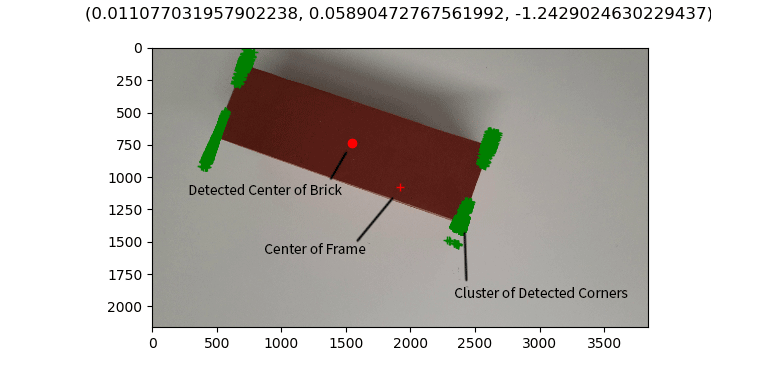
Final image with the angular and cartesian offsets

Finally the x error, y error and angular offset are returned to the path planning algorithm and kinematic model. If the algorithm is unable to find any corners, the code has an exception to the returned error message and will return an array of zeros instead.

How The Path Planning Algorithm Works

The path planning function takes 3 dimensional start and end coordinates as input. The number of steps for each part of the path is soft coded to allow for motion smoothing.

def plan_path(start, end):
number_of_steps_curve = 30
number_of_steps_drop = 20
lowering_height = 0.3
path = np.zeros((number_of_steps_curve + number_of_steps_drop,3)) # initialise array of zeros
step_xyz = [0,0,0] #initialise step

It interpolates the difference in the x and y coordinates linearly. The z coordinate is interpolated along an exponential function so that the brick is always lifted directly upwards from the ground.

for i in range(1,(number_of_steps_curve + number_of_steps_drop)): #incrememnt x and y path according to step_xyz
if (i <= number_of_steps_curve):
    path[i,0] = path[i-1,0]+step_xyz[0]
    path[i,1] = path[i-1,1]+step_xyz[1] 
    path[i,2] = ((i**(1./3)) / ((number_of_steps_curve-1)**(-(2./3)))) * (step_xyz[2]) #incremment z path according to curve equation
else:             #keep x and y the same
    path[i,0] = path[i-1,0]                     
    path[i,1] = path[i-1,1]
    path[i,2] = path[i-1,2] - (lowering_height / number_of_steps_drop)   #lower z according to drop heightp

The graph below shows the x, y and theta values changing linearly and the z value changing as an exponential funciton.

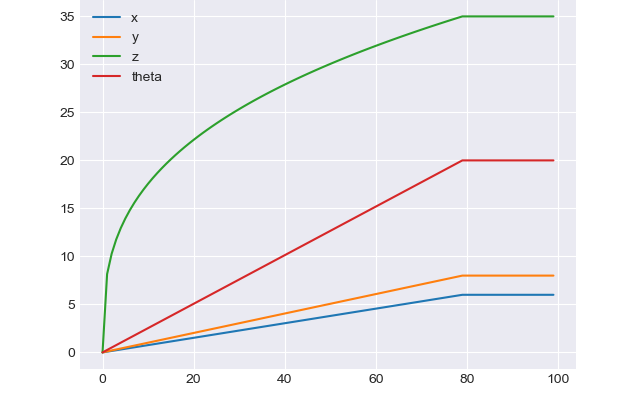
Cartesian coordinates and angle plotted against number of steps